Transit Assignment
Overview
The transit assignment in GTAModel V4.0.1 is done with a congested fare based transit assignment using EMME 4.2.1+. Boarding levels (available in EMME 4.2+) were also utilized to remove walk all way trips from being allowed in assignment.
Integrated Transit Assignment Model
To predict path choices adequately in the presence of competing services with different characteristics and fares one must capture the different factors as best as possible in the path choice process. While many approaches to this problem are conceivable, the decision for operational implementation reasons to use a standard aggregate assignment package (in this case Emme), somewhat limits options. In the current model system the following features are implemented:
- Given that qualitative, unobserved attributes will influence path choice in the heterogeneous integrated network, an “all-or-nothing”, deterministic assignment is not appropriate for this application. The Emme stochastic, multi-path assignment procedure is used. This permits flow for a given O-D pair to distribute probabilistically across competing paths.
- Mode and agency specific boarding penalties are used to capture, at least crudely, differences in reliability or other qualitative “disutility” components of competing services. These penalties are incurred by passengers every time they board any transit vehicle. These penalties seek to discourage passengers from excessively transferring between vehicles.
- Transit users are not restricted to accessing the transit line(s) that directly connect to their access and egress centroid connectors. Instead, they are allowed to “walk on the street network” to access more distant (but potentially more attractive) transit lines. For example, a traveller may “walk past” a bus line to a more distant subway station if the resulting connection is the more attractive one. This feature is particularly useful for modelling travellers originating near “fare-boundaries”, where walking a single block can halve the out-of-pocket cost of a trip.
- Path choice is based on a generalized path impedance function that captures both time and cost effects in the path choice.
- On-board “congestion penalties” are used to capture differential crowding effects on computing routes. Converts the unitless congestion penalty from the conical delay function into weighted time, such that it can be included in the generalized cost function.
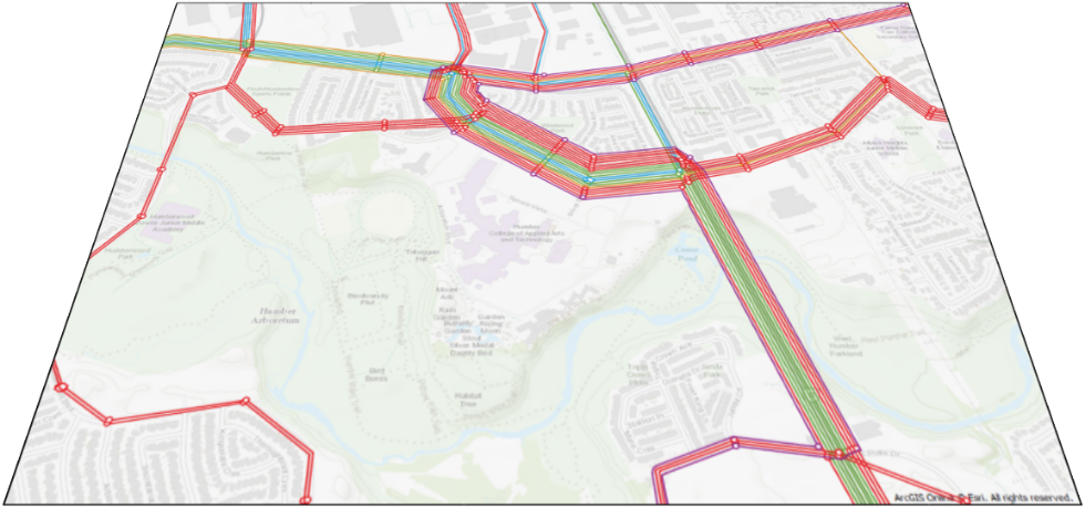
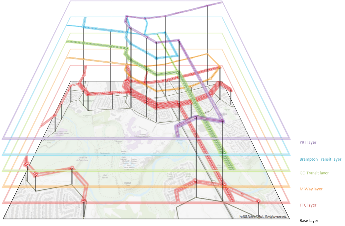
In order to do generalized impedance path choice a “fare-based” procedure was developed in which the base transit network is automatically reconstructed as a hyper-network (see Figure 1.1), in which transfer links between services that involve a fare payment are inserted into the network. Based on their value of time, transit riders “pay” an initial local fare in terms of equivalent minutes of travel time as they traverse the centroid connector connecting their trip origin centroid to the network; they then pay appropriate transfer fares when transferring from one service to another. Distance-based fares, if they exist, are accumulated as the rider travels along a route. Zone-based fare increments are accumulated as the rider crosses a zone boundary. While possibly not able to handle all conceivable fare systems, the current approach does address a wide range of fare policies and is adequate for modelling current and anticipated fare systems in the GTHA.
Transit Time Functions
Each transit line segment has a standard attribute of a transit time function (TTF). During assignment, a congestion term is temporarily added to the transit time function. This congestion delay function is described below.
Congestion Delay Functions
Many transit lines in the GTHA are over-crowded, leading to degraded service levels and poor reliability. If this is not accounted for in the path choice process the model may over-assign trips to popular but over-crowded routes and not capture “spill-over” to parallel competing paths. This may also lead to under-estimation of the impacts of transit capacity improvements on transit ridership levels. To capture at least a first-order sensitivity to crowding effects, the model uses the Emme congested transit assignment procedure. This procedure is the direct analogue to the standard road volume-delay function approach to modelling roadway congestion. In this case the conical volume-delay function is used, with different functions being used for heavy rail (commuter rail and subway), light rail (streetcars and LRT), local buses and regional buses (i.e. GO).
TODO
The exponent term (α) is estimated during the PSO procedure, described in section 2.0. In total, 5 exponent terms are estimated, one for each of the 5 different TTF functions (for various services/modes). The weights for all TTFs are fixed at 1.
Data of Transit Demand
Transit estimation and calibration uses the 2011 Transportation Tomorrow Survey (TTS) data. TTS is a very large (5%) household telephone-based survey that collects weekday travel data for a random weekday all members of sampled households 11 years of age or older. It has been conducted every five years since 1986, with the most recent survey being undertaken in 2011/12. In 2011 118,280 households were surveyed within the GTHA, providing an exceptionally rich dataset for detailed activity/travel modelling. Although a trip-based survey, the dataset was converted for modelling purposes into a set of out-of-home activity episodes describing personal activity patterns and trip chains (tours) for all observed persons.


Estimation and Calibration
Transit assignment parameters were estimated using a Particle-Swarm Optimization procedure. The root-mean-square-error (RMSE) between predicted and observed transit line boardings jointly across the AM and PM time periods is minimized using the aforementioned procedure. That is, parameters were chosen to minimize the following function:
TODO
The values of the behavioural parameters are encouraging, falling within expected bounds. The estimated wait time perception of 2.67 is only a little higher than the industry rule of thumb of 2.5.
Walk perceptions in the model are stratified by 5 different link types:
- Toronto Access Perception applies to centroid connectors within the City of Toronto
- Non-Toronto Access Perception applied to all other centroid connectors
- CBD Walk Perception applies to non-connector links within the boundaries of the Central Business District (an important distinction as downtown Toronto is home to the PATH system of underground walkways linking Union station with much of the financial district)
- Toronto Walk Perception applies to all non-CBD, non-connector links within the City of Toronto
- Non-Toronto Walk Perception applies to all other walk links in the network
The idea behind breaking the walking perception down in this manner is to model the impact that land use and built form have on attractiveness of walking. The City of Toronto developed much earlier than its surrounding municipalities, with visible differences in road layouts and density – even in its more-suburban outer fringes.
Parameter Calibration
After estimating the transit assignment parameters by optimizing the prediction of transit line boardings across the network, the parameters were further calibrated to match as best as possible other key model outputs. Hand calibration was required as the RMSE function is mathematically dominated by individual lines that have high ridership, such as subway lines. This calibration involves a multistep process. At a high level, the calibration procedure consists of:
- Matching agency-specific (and mode specific) model boardings for the AM and PM periods to TTS data.
- Ensuring accurate transfers between agencies based on TTS data.
- Matching metro-to-metro transfers within Toronto to TTS data.
- Observing that walk-all-way trip numbers were within acceptable standards.
Walk-all-way trips: The model predicts that some short trips will “walk all-way” rather than board a transit vehicle. A small number of such trips is deemed to be acceptable. Calibration involved adjusting agency-specific boarding penalties in order to match model boardings to TTS boardings. A ‘good match’ between modelled and TTS boardings, were within an absolute value of 6000. This metric was further expanded to consider the total boardings for the specific mode (by agency), i.e. the relative difference in trips observed and modelled. Boarding penalties were capped with a maximum and minimum value of 10 and 0 minutes respectively. In addition to matching boardings by agency, attention was paid to ensure that transfers between operators were accurate, relative to TTS data. It was critical to ensure that agency-specific initial boardings and final alightings were accurate. Successful model calibration was further predicated on observing accurate metro-to-metro transfers were observed at key interchanges within Toronto. A key interchange is the meeting point of the Yonge University Spadina line and the Bloor-Danforth line. Observing the trips south of Yonge and Bloor was a critical step during calibration. Finally, metro station-specific boardings and alightings were compared to data provided by the TTC.
TODO
Table 4: Predicted & Observed Boardings by Agency, AM & PM Peak Periods presents predicted and observed boardings by transit agency. In general the results represent a very good fit to the observed data and, in our experience, are very comparable to or better than those obtained for other Emme aggregate transit assignment models for the GTHA.
Table 2.4 presents a “transfer matrix” that displays the differences between predicted and observed transit trips by original boarding and final alighting services for the AM-peak period. The top left corner cell highlighted in yellow contains the total number of “walk all-way” trips predicted by the model: i.e., trips that were observed to take one or more transit lines but in the model simply walk from origin to destination. These include trips between adjacent zones that simply travel from an origin zone centroid connector to the destination zone centroid connector, but they also include people walk short distances “on the road network” when the assignment algorithm find this to be the optimal path for the trip maker. The remainder of the first row of the table shows the difference between predicted and observed first boardings by transit service, while the remainder of the first column similarly shows the difference between the predicted and observed last alightings by transit service. The rest of the cells in the matrix show the differences between predicted and observed counts by service of first boarding and service of last alighting as an indicator or the extent to which the transit assignment algorithm is dealing with flows through the multi-agency hyper-network. In general the results are quite good, with the biggest errors again occurring for TTC bus. The TTC bus network, however, is quite a dense, largely grid network of routes within which many feasible, typically competitive paths generally exist and so it is to be expected that the assignment algorithm may display a bit of “confusion” in its selection of paths relative to the observed behaviour.
Finally, the following pages compare predicted and observed boardings and alightings by station for the AM and PM-Peak periods for TTC subway Lines 1, the Yonge-University-Spadina subway line and Bloor-Danforth line, 2. As can be seen from the figure, the model in general does a good job in reproducing the station boarding/alighting patterns along this key component of the network.
TODO